AWA: Academic Writing at Auckland
A Design is a key task in technical, scientific and applied disciplines. The writer creates and evaluates an original solution, often to a real-world issue requiring a practical solution. While there are many kinds of Design papers, in technical and scientific disciplines, Designs tend to include an introduction which explains the purpose of the design, a central section which describes the design and supports this with technical data, and a final section which reviews procedures and shows how the design meets specifications (Nesi & Gardner, 2012, p. 183-185). In AWA, Designs include workplace-type texts, including Lesson and Teaching Plans, which use a different structure.
Title: Optimising the Air Traffic Control Roster at Auckland Airport
|
Copyright: Anonymous
|
Description: You have been asked to look at the rostering of Auckland Airport air traffic controllers. 1) How good are the current staffing levels? 2) Analyse the data to understand flight arrival and departure numbers at different times. 3) How can the current staffing levels be improved to increase roster efficiency and cost effectiveness? 4) You should also ensure your roster satisfies employment law requirements.
Warning: This paper cannot be copied and used in your own assignment; this is plagiarism. Copied sections will be identified by Turnitin and penalties will apply. Please refer to the University's Academic Integrity resource and policies on Academic Integrity and Copyright.
Optimising the Air Traffic Control Roster at Auckland Airport
OPTIMISING A WEEKLY ROSTER FOR AIR TRAFFIC CONTROLLERS AT AUCKLAND AIRPORT
AbstractAuckland airport sees hundreds of aircrafts every day, these aircrafts are under strict control by Air Traffic Controllers during their take-off and landing periods. Guiding these aircrafts in and out of Auckland Airport is an extremely stressful and cumbersome task, it also has a very high risk associated with mistakes made while guiding aircrafts. For this reason, it is of interest to create an efficient and cost effective weekly roster for Air Traffic Controllers to ensure they are working under desirable conditions and minimise the risk associated with their line of work. As a group, we have retrieved data on flight arrivals and departures at Auckland Airport (FlightStats, 2017), using optimisation tools such as excel, Opensolver (Mason, 2017), and Gurobi (Gurobi Optimization, Inc., 2017), we have been able to analyse this flight data and generate an effective and cost efficient weekly roster for Air Traffic Controllers at Auckland Airport. This roster will require approximately 30 Air Traffic Controllers working an average shift length of 5.8 hours. The proposed roster will cost approximately 65,000 NZD.
ContentsAbstract.................................................................................... 1 Glossary of Terms...................................................................... 2 Introduction............................................................................. 3 Aim......................................................................................... 3 Introduction............................................................................. 3 Method.................................................................................... 3 Developing a plan..................................................................... 3 Retrieval and processing of flight data......................................... 4 Shift optimisation model............................................................ 4 Shift Allocation model................................................................ 5 Simulation............................................................................... 7 Adjustment of our roster based on the simulation results............... 7 Assumptions............................................................................ 8 Results and Discussion.............................................................. 9 Conclusions............................................................................ 10
Glossary of TermsATC: Air Traffic Controller RHS: Right hand side
IntroductionAimIn this project, we have tried to create an efficient roster for Air Traffic Controllers at Auckland Airport. In making our roster we have tried to minimise the staffing costs and cost of delaying flights while still ensuring reasonable working conditions for the Air Traffic Controllers and reasonable wait times for flights.
IntroductionWorking as an ATC is a highly stressful job and requires high levels of concentration for long periods of time. It is common for ATC’s to be in control of up to three aircrafts at a time, the risk associated with mistakes in guiding these aircrafts is very high and therefore it is desirable to minimise stress levels for ATC’s. Methods of reducing stress can include but are not limited to; reducing shift times, large rest periods, frequent breaks, and shorter night shifts. It is also in the interest of Auckland Airport to maximise their profit margins, this can be done by reducing staffing costs for ATC’s and avoiding the delaying of flights. The purpose of this project is to create a roster for ATC’s over a typical week period, which minimises the total combined cost of staffing ATC’s and delaying flights.
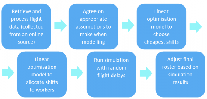
MethodDeveloping a planBefore beginning our project, we had to first discuss how we would approach the problem. This included; deciding what assumptions could be made to simplify the problem, how we should model the problem, where we would get our data from, and how to test our results validity. In the end, we agreed on the following process.
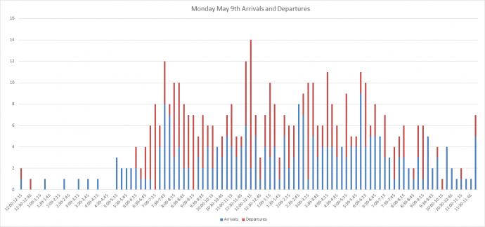
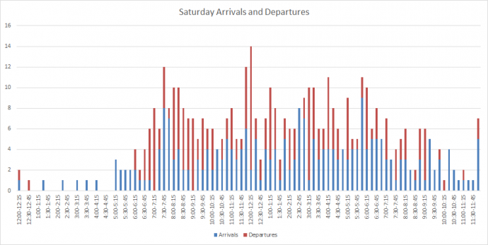
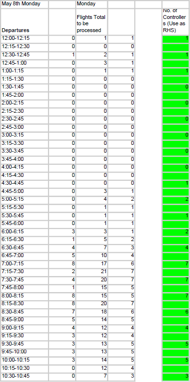
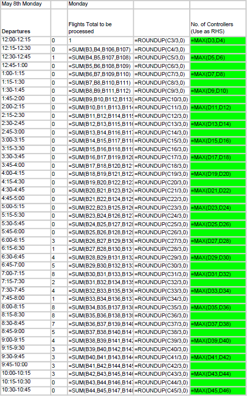
Retrieval and processing of flight dataThe first step in our solving process was to collect data. We did this by hand from a flight stats website (FlightStats, 2017). This was categorised by incoming flights and departing flights, we included both domestic and international flights in our model. The next step was to organise these flights by time, we chose 15 minute intervals as this provides a high level of accuracy without creating too large of a problem. A summary of this data can be seen in figures 1 and 2. After our data was collected we had to process this into usable constraints for my first model. After extensive research into landing and take-off procedures, we determined that flights had to be under control of an ATC during taxiing and take-off/landing (where take-off and landing are defined as the plane being sub 1500ft) for a maximum of thirty minutes. This means that an ATC in any given fifteen-minute period must be concerned with both flights arriving and departing in that period, plus the flights arriving in the previous period, and the flights departing in the next period. Mathematically this gives: ð¹ð‘™ð‘–ð‘”â„Žð‘¡ð‘ ð‘¢ð‘›ð‘‘ð‘’ð‘Ÿ ð´ð‘‡ð¶ ð‘ ð‘¢ð‘ð‘’ð‘Ÿð‘£ð‘–ð‘ ð‘–ð‘œð‘›ð‘› = ð‘‘ð‘’ð‘ð‘Žð‘Ÿð‘¡ð‘¢ð‘Ÿð‘’ð‘ ð‘› + ð‘‘ð‘’ð‘ð‘Žð‘Ÿð‘¡ð‘¢ð‘Ÿð‘’ð‘ ð‘›−1 + ð‘Žð‘Ÿð‘Ÿð‘–ð‘£ð‘Žð‘™ð‘ ð‘› + ð‘Žð‘Ÿð‘Ÿð‘–ð‘£ð‘Žð‘™ð‘ ð‘›+1 Where ð‘› is the ð‘›ð‘¡â„Ž fifteen-minute interval. We then divided the total number of flights under ATC supervision by 3 (and rounded up where appropriate) because our project brief states that one ATC can supervise 3 flights at once. A possible weakness of the process is that it assumes that flights will need to be supervised for the full thirty minutes, when in reality it may range from fifteen to thirty minutes. While this may result in a slightly inflated requirement of ATC’s, it will never understaff, this was chosen to be the preferable method for this reason. The spreadsheet that processed this data is shown in figures 3 and 4.
Shift optimisation modelThe purpose of this model was to choose the cheapest combination of shifts while still meeting the demand for ATC’s. I chose to model this as a transportation problem. In the model, each shift pattern was represented as a series of ones and zeros, where a one implies there is an ATC on during that time period, and a zero indicates that there is either no ATC’s working or an ATC is on break. This is shown in figure 6. We decided that workers would not want to work a shift less than 5 hours, so I used this as our minimum length shift. Our research into labour laws for ATC’s indicated that they can not work shifts greater than 10 hours (this can be extended to 11 hours with approval from the ATC) so I chose shift lengths of 5, 6, 7, 8, 9, and 10 hours. The labour laws for ATC’s also state that ATC’s must have breaks at least every 2 hours for a minimum of 30 minutes, for each shift length I implemented a shift pattern that had breaks every 2 hours and one with breaks every one 1.5 hours. I also decided it was suitable for workers to start and finish at half hour intervals, this resulted in 6 shift lengths X 2 shift types X 48 starting times = 576 unique shift patterns. Our research indicated an appropriate ATC wage is approximately $75/hour, this is the wage we used for our model, we also included an overtime wage of $150/hour for every hour worked over an eight-hour shift, this complies with the ATC labour laws. I analysed the data we had collected and determined a typical week of flights would require approximately 1300 hours of ATC work, assuming an ATC will work around 40 hours a week, 1300/40 ≈ 31, so a suitable cap on the number of workers is 40. If all 40 workers all worked 5 shifts a week results in a maximum of 200 shifts that can be worked. Because of this I introduced a constraint that the total number of shifts must be less than 200, this constraint is necessary because the solver avoids the 9 and 10 hour shifts as they are more expensive per hour than the shorter shifts, in practise this would require the airport to hire more ATC’s, while it would actually be more practical and cost effective to extend current employees shifts for an unusually busy week. The overall objective for this function is to minimise the cost of staffing, mathematically this is represented by The cost associated with each shift is calculated by subtracting breaks from the shift length and then multiplying by the hourly wage of $75/hour. A partial solution from the shift optimisation model is shown in figure 8.
Shift Allocation modelThe purpose of this model was to use the shifts determined by the shift allocation model and distribute them among workers over a one week period. I modelled this as an assignment problem where shifts had to be assigned to one of 40 workers. The most important constraint in this model is that each shift has to be assigned to a worker, there cannot be less shifts assigned as this would fail to meet the demand for ATC’s, and there cannot be more shifts assigned as this would not be using the most cost effective option. However, there are several labour laws that must be followed when rostering staff; I have broken down these laws and how I incorporated them into the model below. Figures relevant to this model and its constraints are figures 9, 10, and 11
1 A shift is considered a night shift if the ATC works partly or wholly within 1:30 am – 5:30 am
The objective for this model was to assign all the shifts to the least number of workers possible. This was done by assigning each worker a weight where worker 1 has a weight of 1, worker 2 has a weight of 2, and so on. The total number of hours each ATC was working was multiplied by their weight and then summed together, this value was to be minimised.
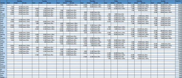
Once the solution was generated it had to be converted into a more readable format, I used Excel to automatically generate a roster based on the models solution. The roster shows each worker’s start and finish time for every day as well as their breaks, it is automatically updated after each sequential solve of the model. The final roster can be seen in figure 12.
SimulationThe first step in making our simulation was to find out how common it is for flights to be delayed and how long they’re delayed for. We used a flight statistics website (FlightStats, 2017) to obtain data on how many flights were delayed more than 15 minutes, we felt that this wasn’t too large of a bracket and decided to use a combination of this data and data retrieved from a second website (Air New Zealand, 2017). Using all of this data we calculated a rough probability of a flight being delayed by 15, 30, or 45 minutes (early flights and flights later than 45 minutes were excluded due to infrequent appearance). The probabilities used are shown in figure 13, and a partial screenshot of the simulation in figure 14. Once these probabilities were calculated we used a binomial distribution based on these probabilities to estimate how many flights would be delayed in each 15-minute period (arrivals and departures). Using the numbers produced by the binomial distribution we calculated how many flights needed to be served in each 15-minute interval. This is done by a summation of flights that arrived on time during that period, flights that should have arrived in the last period (but were 15 minutes late), flights that were scheduled two periods ago (but were 30 minutes late), and flights that should have arrived three periods ago (but were 45 minutes late). The above process was then repeated for departing flights. Once all the calculations were complete we computed ð‘›ð‘¢ð‘šð‘ð‘’ð‘Ÿ ð‘œð‘“ ð‘“ð‘™ð‘–ð‘”â„Žð‘¡ð‘ ð‘Žð‘Ÿð‘Ÿð‘–ð‘£ð‘–ð‘›ð‘” + ð‘›ð‘¢ð‘šð‘ð‘’ð‘Ÿ ð‘œð‘“ ð‘“ð‘™ð‘–ð‘”â„Žð‘¡ð‘ ð‘‘ð‘’ð‘ð‘Žð‘Ÿð‘¡ð‘–ð‘›ð‘” − 3 ∗ ð‘›ð‘¢ð‘šð‘ð‘’ð‘Ÿ ð‘œð‘“ ð´ð‘‡ð¶′ð‘ ð‘Ÿð‘œð‘ ð‘¡ð‘’ð‘Ÿð‘’ð‘‘ ð‘œð‘› for each 15 minute interval, this gives us the number of flights that could not be served in each period. The next step was to write a macro that would repeat the simulation 100 times and paste the number of flights that were not served in each period into a separate spreadsheet. The VBA code to do this is shown in figure 15. From this sample, we were able to calculate a mean number of unserved flights and a 95% confidence interval for each period.
Adjustment of our roster based on the simulation resultsUnserved flights cost the airport money and are an unnecessary nuisance for the passengers, however it is not always favourable to have more ATC’s on to avoid this. We tackled this by trying to find the cheapest combination of hiring extra ATC’s and letting flights go unserved. We did this by calculating the fuel cost for running a plane for 15 minutes. We recognise this is a very rough estimate, however this is not a crucial part of the model and we could not find a better statistic online. We estimated that the cost of delaying a plane for 15 minutes is $309, this cost was multiplied by the mean number of unserved flights for each period, then divided by 3 so it could be compared to the cost of hiring an extra ATC. Once this was complete we used excel to find the 30 periods with the highest cost due to unserved flights. At this point I decided to propose two different options; resolving the models, or manual adjustment of the roster, I have broken down the intricacies of both options below. Resolving the modelsAfter finding the periods with the most unserved flights, we can increase the demand for ATC’s in the required periods in the shift optimisation model, this can then be resolved and then create a new roster based on the new demand values. This option is likely more cost effective, however I found that it would not be as practical as the following option.
Manual adjustmentI have included an identical but blank roster immediately below the roster produced from the solver, once we know what periods will require more ATC’s, I can manually enter extra shifts into the empty roster, alternatively, I can enter a -1 or 1 into the blank roster to adjust a worker’s shift to start an hour earlier or go for an hour longer respectively. A third roster then prints the updated shifts with the original shifts in one place. I felt that in practise, this method would be more useful. This is because in the real world it is likely for the airport to run a simulation for every week, resolving the model based on every simulation result would lead to a different roster every single week, this is not practical for workers. I believe it is more likely for a manager to instead offer extra shifts to ATC’s based on the simulation results, and then enter the extra shifts manually, this way ATC’s can expect a regular roster and have the opportunity to acquire extra hours. The disadvantages of this method are that the manager has to carefully check that they are not breaching any labour laws when they are entering or extending shifts, it is also not as cost effective and requires more effort compared to resolving the model.
We chose to use the manual adjustment option. Our simulation resulted in two periods where the cost of unserved flights was greater than the cost of hiring an extra ATC for 5 hours. Coincidentally, these periods could both be handled by introducing a single extra shift, we added one ATC who will work from 7:00 – 12:00 am on Saturday with breaks every 1.5hrs. The introduction of this extra shift saved a total of $680.
AssumptionsWe made several assumptions throughout our modelling process with the aim of simplifying the model without compromising our models accuracy. I have listed the assumptions we made in order to model the problem as we have;
Results and DiscussionThe final output from our model was a weekly roster with a total costs breakdown. This output is presented in a table and can be seen in figure 12 Our final solution has the following parameters;
The shift optimisation model I produced takes approximately 5 minutes to initialise and solve with Gurobi. The shift allocation model is much larger, without Gurobi it was left for over 50 hours without reaching a solution, once Gurobi was installed it now takes approximately 2 hours to initialise and 5 minutes to solve. The initialisation stage only has to be performed once when using quick solve, so in practise the entire problem can be solved in under 5 minutes. The results from our simulation are as follows;
Auckland Airport currently uses a system where between 6:00 am and 8:00 pm there is three ATC’s working and one covering their breaks (so there is always three ATC’s working). Between 8:00 pm and 6:00 am there is two ATC’s working (Dempsey, 2017) The real roster and our solution can’t really be compared in terms of cost or efficiency as our solution assumes there is not a maximum capacity of three ATC’s in the tower and that the ATC’s can only control 3 flights at once (as was instructed).
ConclusionsWe were able to generate a cost effective weekly roster that meets the demand for ATC’s at Auckland Airport, however the assumptions used in our model have affected the validity of our solution (specifically the maximum capacity constraint). Our solution is still useful as an approximate roster, under our assumptions, we can conclude that;
We cannot make a recommendation to Auckland Airport due to the restricting assumptions given to us in the project specifications, however, our model will still function and create a roster if the maximum number of flights that can be controlled was increased to a more realistic value.
BibliographyAir New Zealand. (2017, May 28). Retrieved from https://www.aucklandairport.co.nz/flights FlightStats. (2017, May 28). Retrieved from http://www.flightstats.com/go/FlightStatus/flightStatusByFlight.do Gurobi Optimization, Inc. (2017, May 22). Retrieved from http://www.gurobi.com Mason, A. (2017, March 6). OpenSolver For Excel. Retrieved from http://opensolver.org/
Group ContributionsAs a group, we collaboratively developed a process that would produce a solution to the problem presented to us. We worked together to decide which assumptions were valid to make and which were not. We also worked together to estimate a cost of delaying a flight. My role in the group was to decide how to model the problem and create it. Initially I created a 24-hour model but this was exchanged for the other two models I developed to solve the problem over a week. This includes developing the final roster and all the constraints included in the model. I also implemented the simulation that was developed by my group members. .... was responsible for gathering our data (by hand) and sorting it by time interval, he also helped me implement the simulation into the model. Some of this data is shown in figures 1 and 2. .... also did extensive research into labour laws and delay costs, however, these were not used to produce our final solution. .... researched labour laws for ATC’s and I implemented them into the model. ..... was also responsible for analysing flights and determining the delay probabilities used in our simulation. ..... used the flight data gathered by Josh and developed a spreadsheet to process the raw data into a RHS constraint for my models, the data needed to be converted from flights arriving/departing in each interval into number of ATC’s required for each interval. ..... also did most of the work in developing an appendix for us to use for our reports.
APPENDICESGroup 7
(group member names here)
Figure 1: Arrivals and Departures on Monday 9th May
Figure 2: Arrivals and Departures on Saturday
Figure 3: Development of Right Hand Side Constraints Figure 4: Formulation of Right Hand Side Constraints
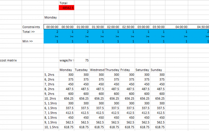
Figure 5: Comparison of output of model to Minimum air traffic controller constaints in blue , the objective function cost figure is shown in red
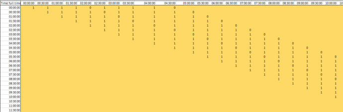
Figure 6: An example of the matrix representing when controllers were on a shift, or not.
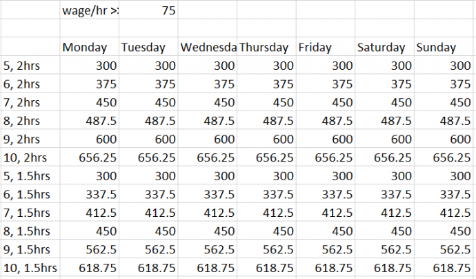
Figure 7: A cost matrix showing the cost of each shift pattern
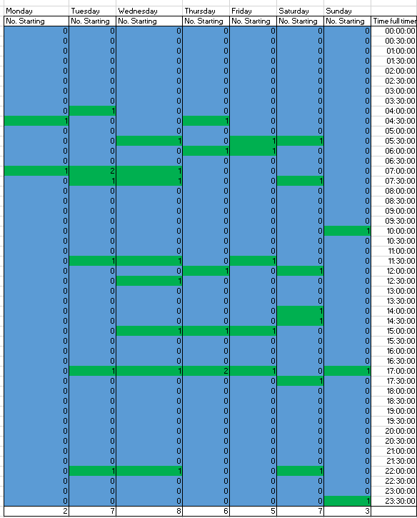
Figure 8: Our solution to the shift model
Roster
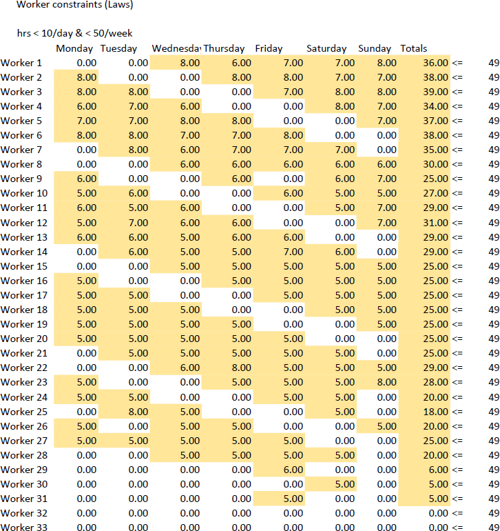
Figure 9: A matrix showing the number of hours each worker is working on each day.
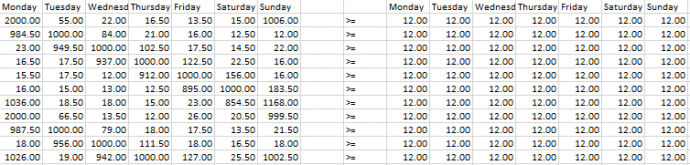
Figure 10: These cells show the enforcement of the labour constraint that there must be 12 hours between shifts
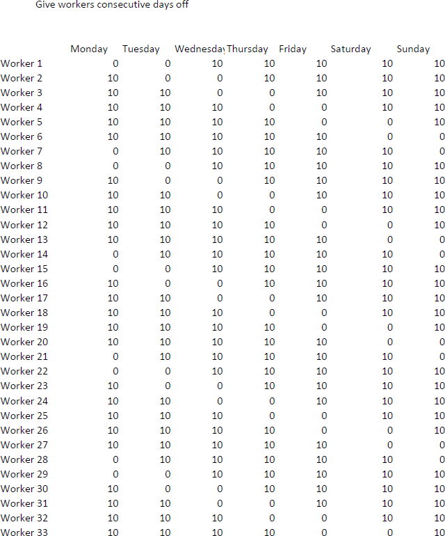
Figure 11: These excel cells show which days of the week workers have guaranteed days off (represented by 0s)
Figure 12: Our final roster
Simulation
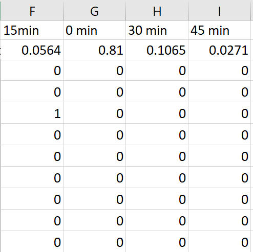
Figure 13: The probability of an on time arrival, 15, 30 or 45 minute delay
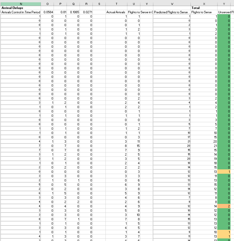
Figure 14: Simulation spreadsheet
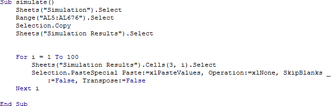
Figure 15: Code used to generate 100 simulation results
Figure 16: Sample of simulation results. |
 where ð¶ð‘– is the cost associated with shift ð‘– and ð‘¥ð‘– is 1 if the shift is selected and zero otherwise. 𑖠ϵ {1,2,3, … ,4032}. A partial screenshot of the objective function is shown in figures 5 and 7.
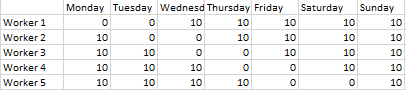
 where ð‘Šð‘– is the weight of worker ð‘–, and ð»ð‘– number of hours worked by worker ð‘– in one week, and 𑖠ϵ {1,2,3, … ,40}.